Raytracing Explosive Liquid
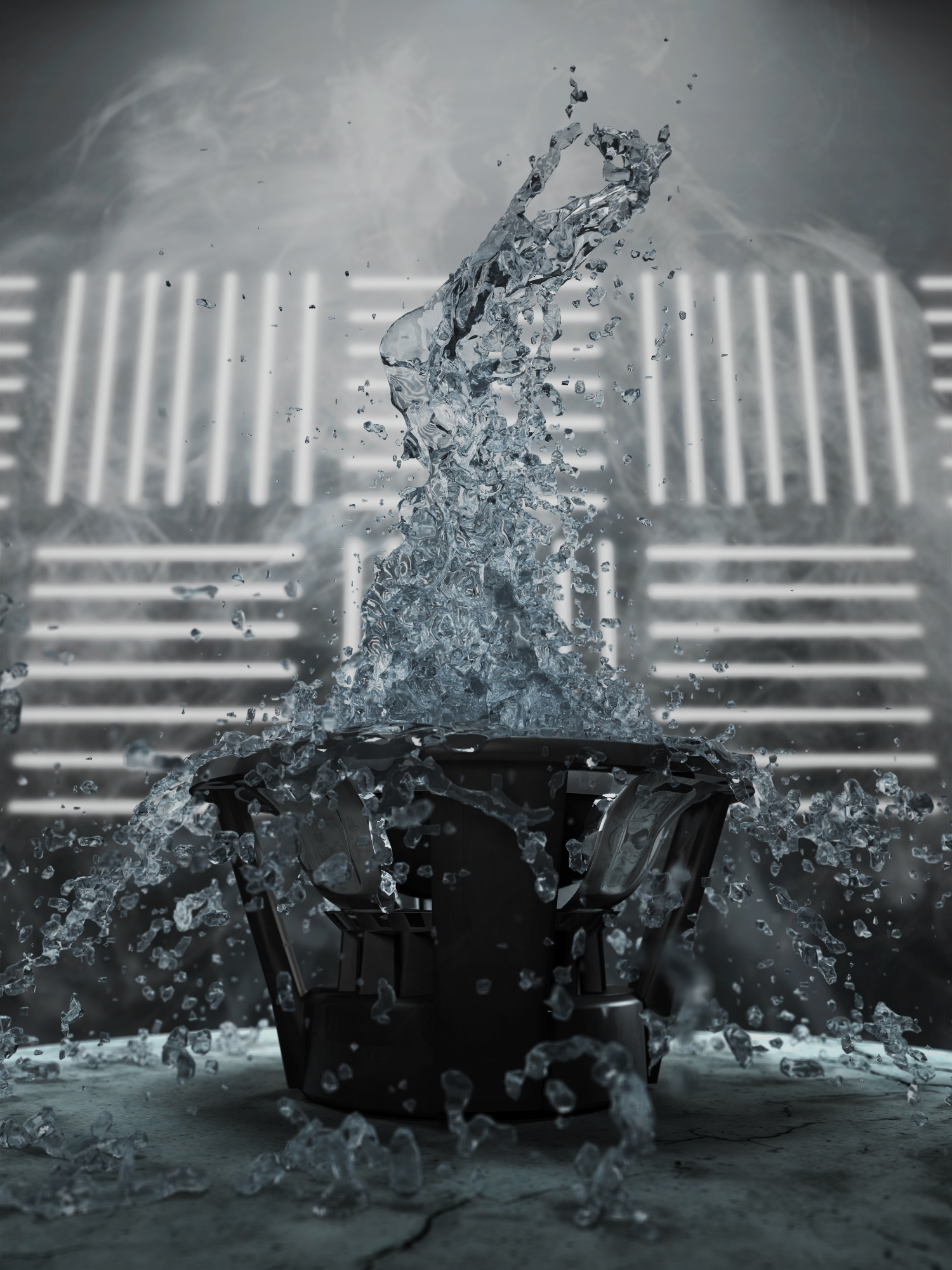
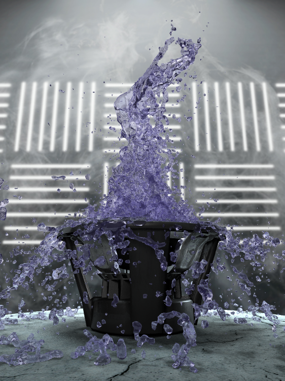
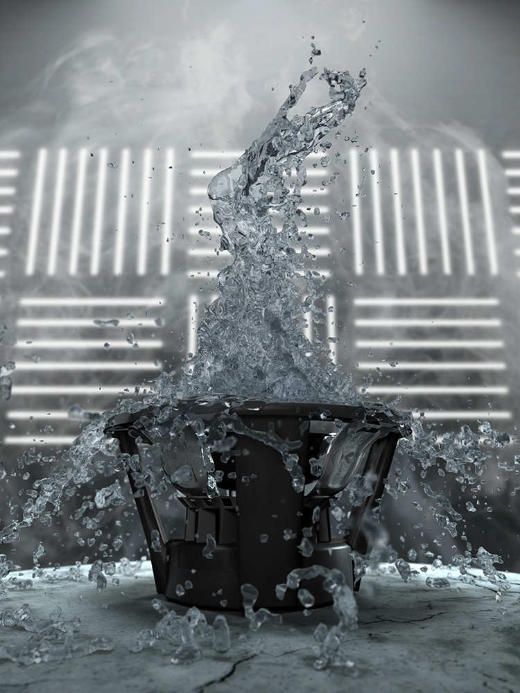
I took Stanford’s CS 148 (Computer Graphics) this quarter. For the course’s final project, we were asked to design a scene and assemble/render it in a raytracer. The following is the image that I created:
I spent about a week on this project. While there is much I could have improved, I am pretty proud of the results, so I wanted to document my process and reflect a little on what I could have done differently.
Background
- CS 148 is Stanford’s first course in its computer graphics track. The class provides an overview of important concepts and techniques used throughout graphics. The first half of the course focused on scanline rendering, while the second half focused on raytracing.
- For those unfamiliar, raytracing is the process of tracing light rays around
a scene in order to produce an image. Wikipedia has a good summary:
In computer graphics, ray tracing is a rendering technique for generating an image by tracing the path of light as pixels in an image plane and simulating the effects of its encounters with virtual objects. The technique is capable of producing a very high degree of visual realism, usually higher than that of typical scanline rendering methods, but at a greater computational cost. This makes ray tracing best suited for applications where the image can be rendered slowly ahead of time, such as in still images and film and television visual effects, and more poorly suited for real-time applications like video games where speed is critical. Ray tracing is capable of simulating a wide variety of optical effects, such as reflection and refraction, scattering, and dispersion phenomena (such as chromatic aberration).
- For the project, we were provided with a basic raytracer implementation, which we then had to modify (if necessary) in order to support effects needed for our scene. The raytracer already supported refractive/reflective materials, which made my life a little easier, but I still needed to implement additional features (detailed below).
- In brainstorming my scene, I was inspired by ferrofluid and non-Newtonian fluid displays, and I thought this video of paint on a speaker was cool. I set out to create some sort of image involving fluid on a speaker.
Modeling in Maya
Trying to figure out the positions/orientations/sizes of meshes, lights, and the camera by guess-and-check in the raytracer is painful (even the low-quality renders took at least a minute or two), so I tried to model my entire scene in Maya first, before importing coordinates into the raytracer and making adjustments there.
I had no prior Maya experience (and very little experience with any other modeling software), so I wanted to build my scene using simple objects that would teach me a bit but wouldn’t suck up too much of my time. I decided to start simple, with just a speaker resting on a table, and there actually isn’t much more than this in my final image.
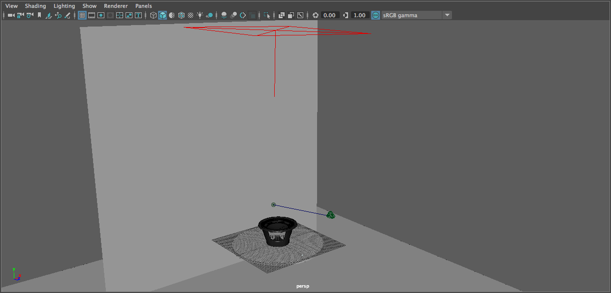
I downloaded a free 3D model of a speaker/woofer from Archive 3D, added a cylinder for a table, and created 2 planes to form the floor and back wall. I imagined a low-key top-lit sort of scene (something like this, but with exploding fluid instead of a creepy dude), so I added a single area light above the table. When creating and placing the camera, I wanted to create a feeling of being “in” the scene, and I wanted the explosion to be emphasized as much as possible. In (real life) photography, I would have used a very short focal length to achieve this effect, so I created a camera with a 20mm focal length and placed it fairly close to the speaker.
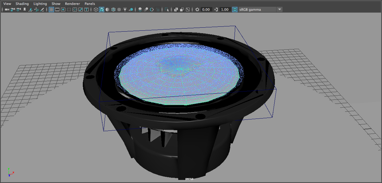
With the basics of the scene set up, I turned to YouTube to figure out how to use Bifrost (Maya’s fluid simulation tool). This took lots of fiddling – so many hours of fiddling. I essentially created a (very) smushed sphere as a liquid emitter and placed it just above the speaker cone, then duplicated/merged the speaker model into a single mesh and designated that as a collider, and made the table a collider. I created a mesh representing just the cone of the speaker (partly by merging objects from the original model, partly by doing a little modeling myself) and keyframed it so that it rapidly moved up and down, and I made this a collider as well. Then I ran the Bifrost simulation a bunch of times, tweaking fluid parameters and the shape of the emitter until I found a particular frame I liked.
This part was so fun to work on, but it was also painful. Maya is incredibly fond of crashing frequently, at both opportune and inopportune times, and the Bifrost simulations took a long time to run. Autosave is pretty intrusive when the “you are broke and are using the student version!” notice appears on every save, so I had to disable it.
That image doesn’t look amazing, but it’s a start!
Once I selected a frame I liked, I generated a mesh from the Bifrost fluid and exported each mesh in my scene to an individual .OBJ file. Time to start working in the raytracer!
Moving to the raytracer
The raytracer is already well-equipped to render most basic scenes, so I was able to load my meshes (via assimp) and produce a draft render without much work. The raytracer implements Blinn-Phong-based shading by default, and I found this to be good enough to create the materials in my scene. (In the class, we discussed the implementation of other shading models such as those used in Unreal Engine 4, but I didn’t think it was necessary to implement this for my materials.)
Two important modifications I made:
- The raytracer already includes an area lighting implementation, but I extended it to support light decay. This was simple; the raytracer calculates an attenuation factor based on the distance to each light.
- The provided raytracer calculates if an object is in shadow by tracing a ray towards each light source and checking if the rays hit an object before reaching the light. I modified this so that if the shadow rays intersect a semi-transparent object, we resume tracing the ray on the other side of the object and calculate some net attenuation based on the transmissivity of the object(s) that the shadow ray passed through. This allows the fluid to cast softer, more realistic shadows.
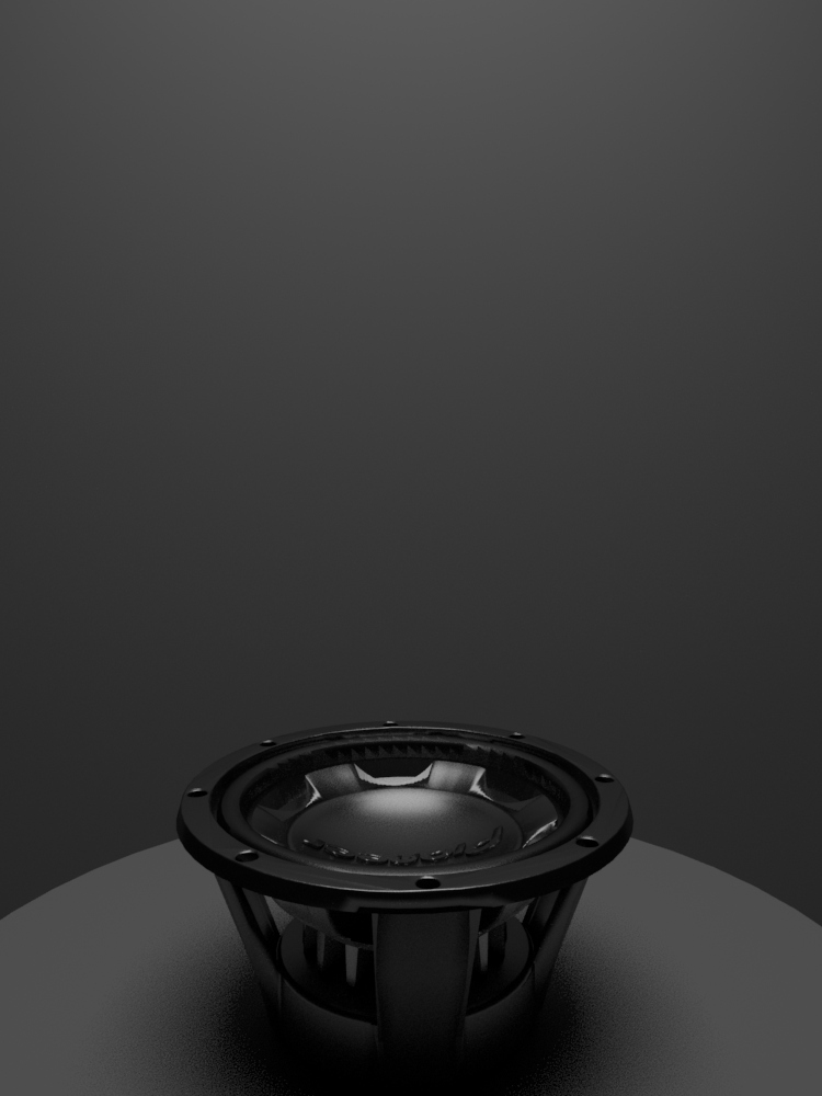
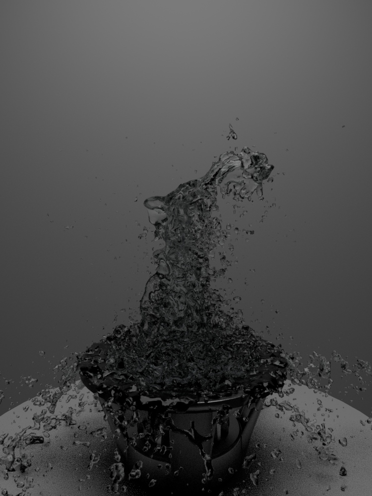
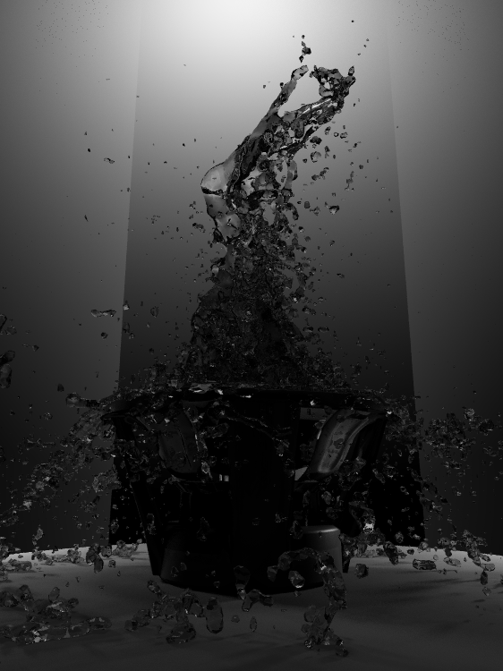
2) Basic raytraced speaker, no modifications to raytracer
3) Basic raytraced scene (with fluid), no modifications to raytracer
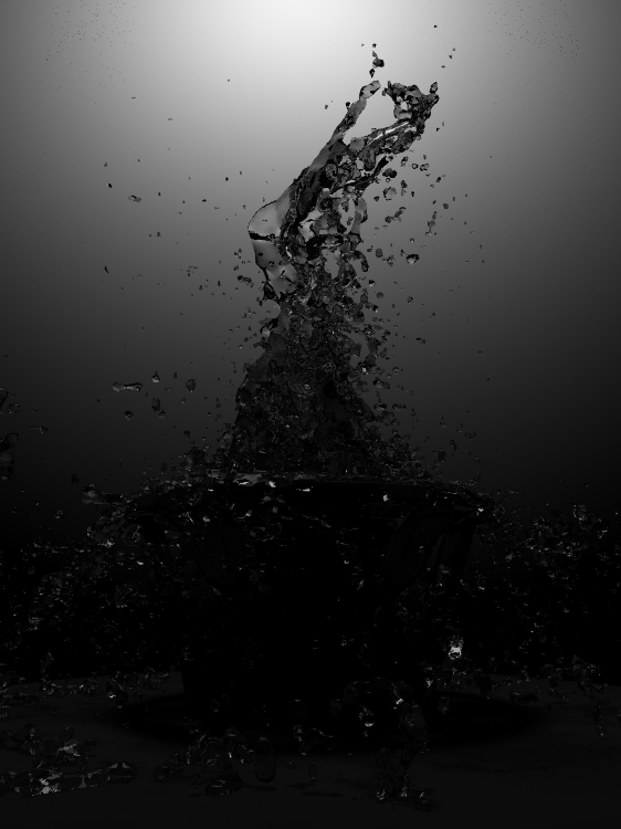
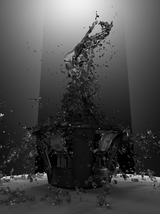
4) After implementing transmissive shadow rays
5) After implementing light decay
Lighting
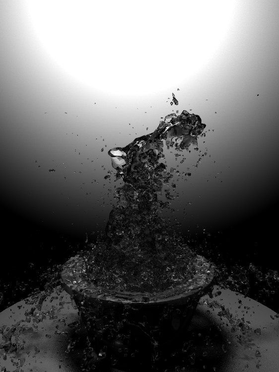
At this point, I started to experiment with ways to make the scene brighter and better-defined. In the above images, it’s almost impossible to tell that the thing on the table is a speaker, and I wanted to find a way to bring it out. I tried several ideas; at some point, I even tried creating a ring light inside the speaker:
It looks kind of cool, but it’s still too dark, and it made the render time blow up.
Eventually, I decided that given the speaker model I was using (doesn’t look that recognizable as a speaker) and the amount of liquid on top of it, it would be difficult to find a way to make the speaker recognizable. It would be fine if the viewer can’t tell that the thing on the table is a speaker, as long as the image looks cool. With that constraint gone, I went back to playing with camera angles. I moved the camera closer to the table, tilted further upwards; this, combined with the short focal length, makes the liquid explosion more prominent in the image.
However, with this angle, it became even more important to give the scene better definition. I tried placing a light directly behind the speaker so as to create a rim light effect, but this didn’t work very well. The outline of the speaker didn’t illuminate as I had hoped; in real life, light would bounce around on the rear side of the speaker and would scatter around the edges, but the raytracer is too simple and the mesh too perfect to reproduce this effect. (I did not implement global illumination, but I don’t think it would have helped here.) Also, the water stayed dark, since it has no diffuse BRDF response. (It may have helped illuminate the water if I had placed a luminous plane – like a softbox – below the plane of the table, so as to appear, refracted, through the water, but I did not try this.) I ended up adding rear-left and rear-right area lights to achieve some degree of backlighting effect, and then I added a front area light to fill in some shadows in the speaker.
Texturing
I wanted to add some smoke and fog to the scene. However, we had been told that implementing participating media well can be extremely challenging, and I was running low on time, so I did this via a background texture. (Is this cheating? Maybe a little bit.)
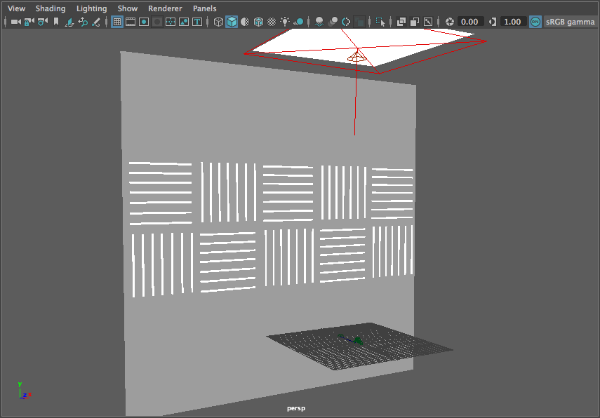
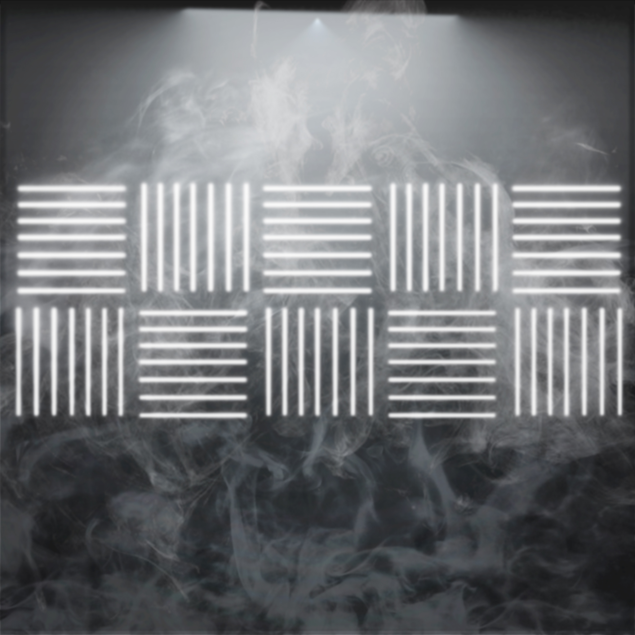
In Maya, I removed everything except for the rear wall and the top area light. I created an Arnold atmosphere volume to produce a sort of fog/dense atmosphere effect (I set the atmosphere density to 0.02 for a subtle effect), and I added a spot light in the same position as my top light so that the narrower “cone” of light from this source would interact more prominently with the atmosphere. I played with the color of the lights, making them very slightly blue. I then created an array of 7 thin, long cylinders, placed right up against the wall plane and shaded with a fully incandescent material, and duplicated this many times to form a grid. I added a front orthographic camera, positioned it such that the wall filled the frame, and rendered this to a 2048x2048px image.
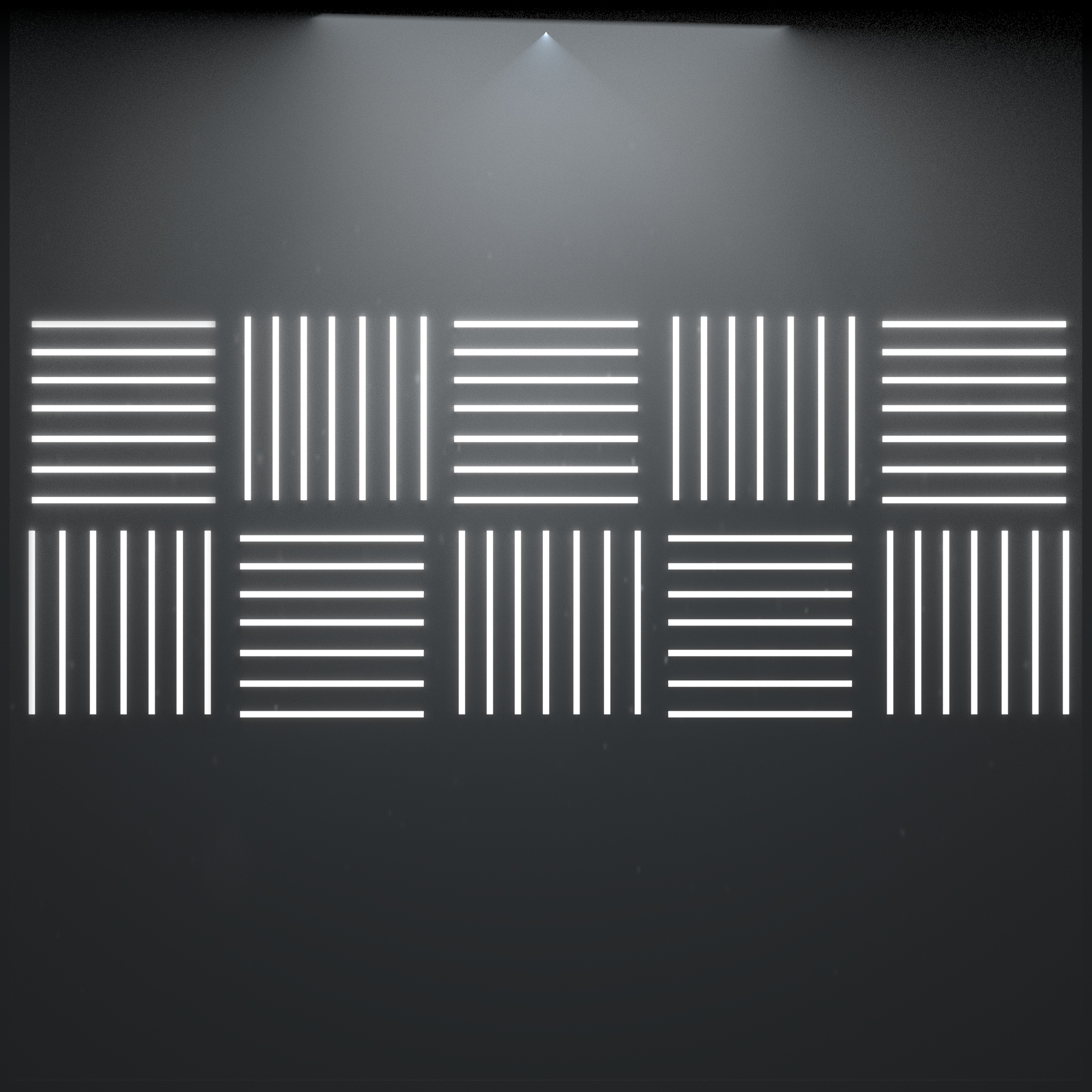
In Photoshop, I composited two fog textures onto the image using soft light and lighter color blending modes. I made several curves adjustments on the fog textures and modified the opacity of the layers until I was happy with the blend. On top of all this, I added two layers simulating an ND linear gradient filter and a vignette effect, then another curves adjustment to brighten up the entire background. I applied a 4px Gaussian blur to the background image (from Maya), then merged all the layers and applied another 2px blur on the resulting image (allowing me to blur the background “lights” more than I blurred the fog, giving the illusion that the fog is closer to the camera).
In the raytracer, I added support for background texturing so that the background plane doesn’t respond to light (I already baked the lighting into the texture itself). Instead of computing a diffuse BRDF response, the raytracer simply samples from the texture image.
For the table, I downloaded a concrete texture and made several heavy curves, hue/saturation, and exposure adjustments in Photoshop. (These adjustments required several iterations of making changes in Photoshop and then checking the results in the raytracer.) I colored the texture slightly blue/green, knowing that was the general color I wanted the scene to have.
More lighting and material adjustments
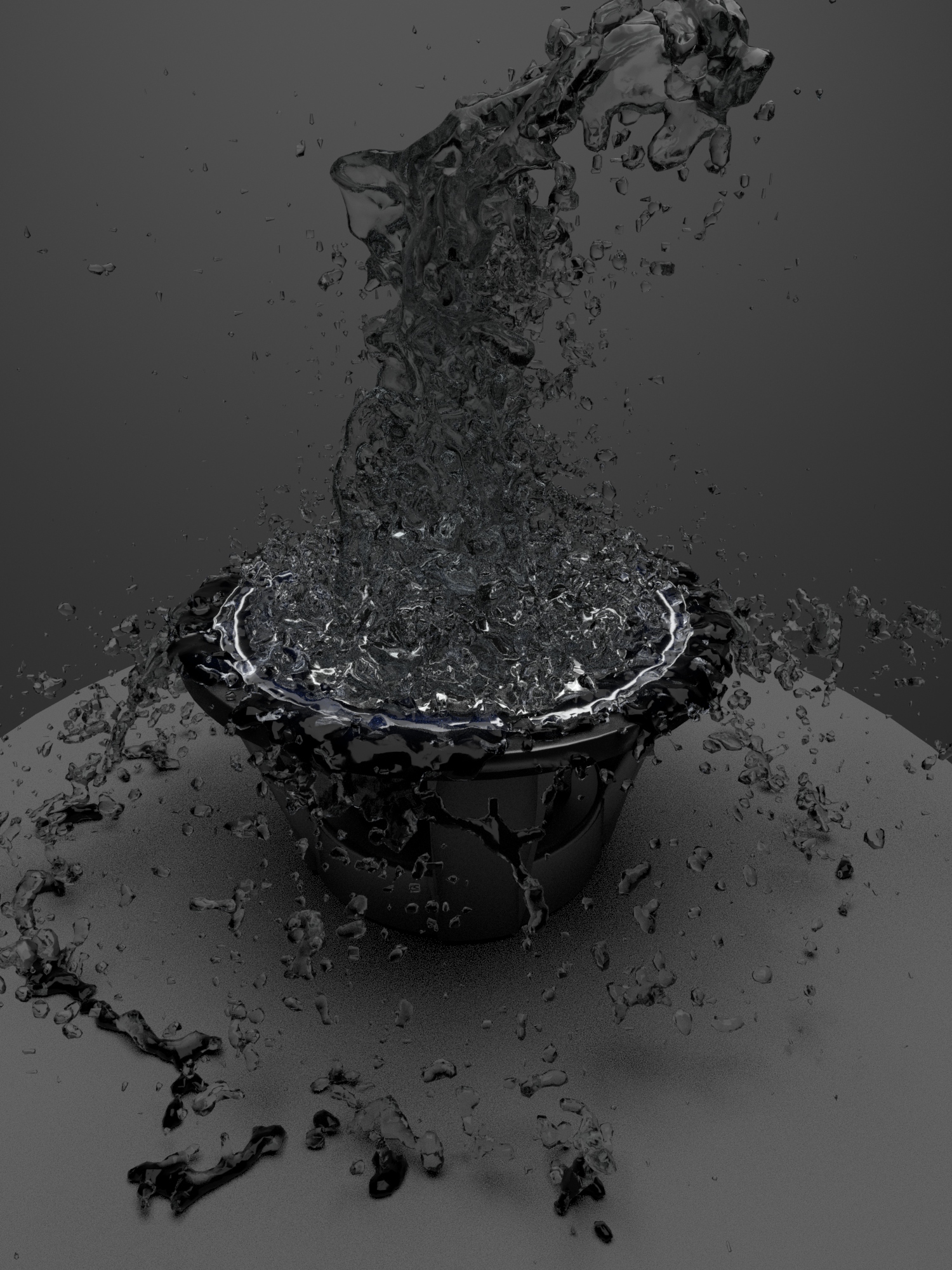
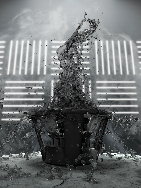
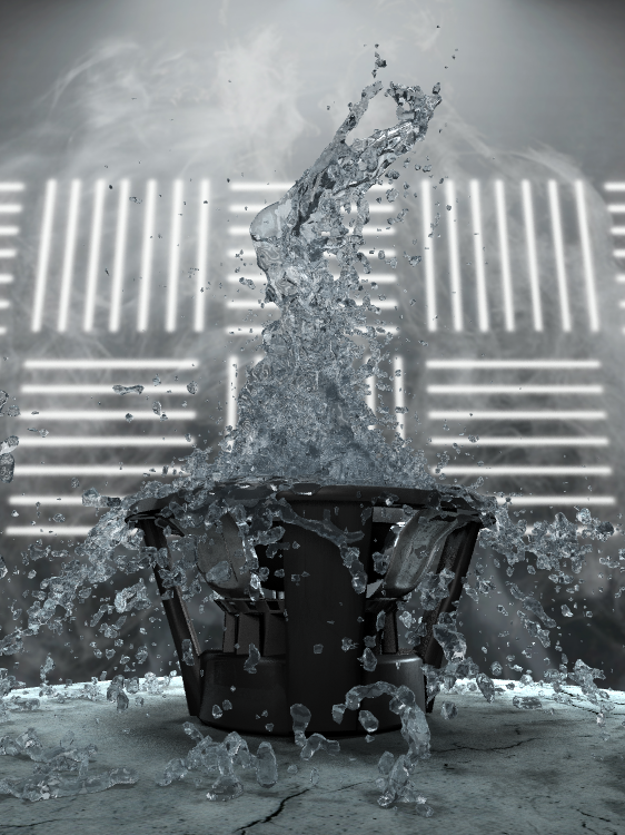
This is starting to come together! I played with the colors of the lights a little bit, looking to give the scene a bluish/greenish cast:
I also wanted to see if I could brighten up and colorize the fluid by adding ambient lighting to the fluid material. I experimented with colors, and even ended up with this craziness at one point (which I quite like):
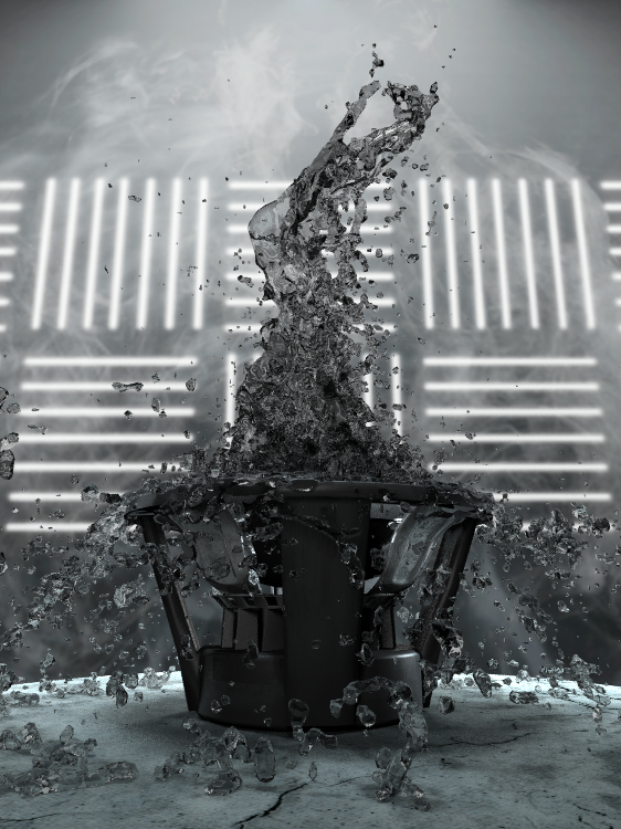
I ended up using this color for my final render, though I wish I had spent a little more time experimenting:
Depth of field
Finally, I implemented depth of field (DoF) in the raytracer for a more photorealistic effect. First, I defined a focal plane (for my scene, at z = 3), which is where the camera is “focusing.” In normal raytracing, for every pixel in the output image, the raytracer emits a ray from the “pixel” on the image plane (the “camera sensor”) into the scene. My raytracer calculates the intersection of the ray and the focal plane – call this the “focus point” – which is shown as the gold circle in the image below.
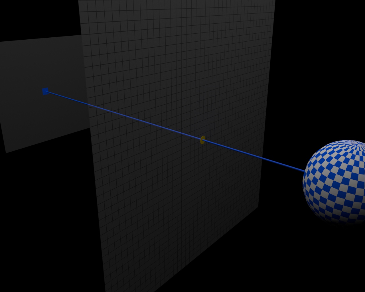
Then, it emits additional rays from surrounding pixels on the “camera sensor” aimed through the focus point, and it traces these rays into the scene.
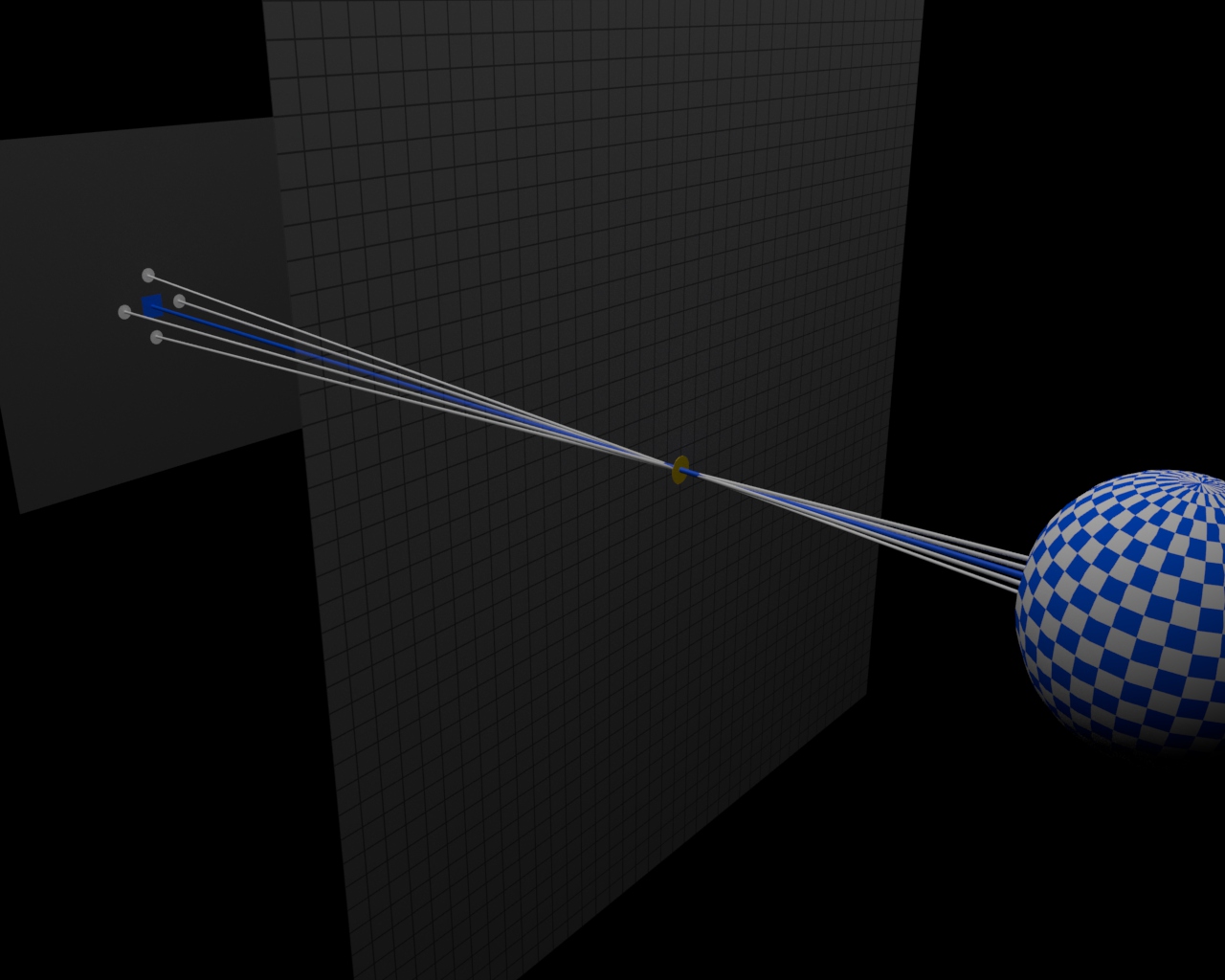
The colors from all the rays are averaged together to determine the final color for the output pixel, and then the raytracer moves onto the next pixel.
If an object is “in focus,” all of the emitted rays for a pixel will converge at the focal plane and will all produce the same color. However, if an object is far from the focal plane (as in the example image above), the rays may intersect several distinct parts of the object (or several different objects entirely), producing a blurry result when their colors are averaged.
The strength of the DoF effect depends on the sampling radius (for each pixel, how far away from that pixel do we generate additional rays?). If the sampling radius is set to 0, everything in the scene will appear in sharp focus, and if the sampling radius is large, objects far from the focal plane will be very blurry.
This approach is comically time consuming. The rendering time increases quadratically with the number of DoF samples per axis, and I had to use higher sample counts (5x5 to 7x7) to avoid aliasing issues. However, it works…
Final adjustments in Photoshop
I added a few small curves and exposure adjustments in Photoshop to finish off the image. Voila!
Parting thoughts
This project was more of an artistic challenge than a technical one – the most difficult technical portion was likely being inventive in parallelizing the render – but it was enjoyable and challenging nonetheless, and certainly helped me better understand the concrete details of building a raytracer.
Render time was a big challenge. It took 67 hours to render the above 2000x1500px image on up to 384 cores at a time. In the later stages of the project, I spent most of my time freaking out about how slow the render was going and trying to find ways to shard the computations across more machines (as well as finding more machines to distribute the computations to). This raytracer has terrible performance. (Technical note: I used OpenMP to parallelize within a single machine, and wrote some scripts to render chunks on the image across many machines.)
Depth of field caused the most significant increase in render time; rendering with an acceptable number of samples creates a 25x slowdown (using fewer samples causes too many aliasing issues). I could have implemented adaptive sampling, where more samples are used to render objects far from the focal plane and only one sample is used to render objects on the focal plane, but I didn’t think of this until the render was already significantly underway. As an even easier alternative, I could have rendered the image without DoF, created a copy with a Gaussian blur applied, and then used a depth map to blend the blurred image with the non-blurred image. This may not be photorealistic, but the DoF in my image is so subtle that there likely would not have been much difference.
Since turning in the project, I also came across other DoF techniques that I would like to explore some day. This article details interesting techniques for creating bokeh (meant for real-time rendering, but worth playing with nonetheless). Again, the DoF in my image is subtle, and I could potentially create a lot more depth in the image by adding more varied light sources with more interesting bokeh.
From an artistic standpoint, I would have loved to have made another attempt at making the image low-key. The image is fairly well lit and departed a lot – maybe too much – from my original idea of a low-key, top-lit (or backlit) image that I described early in this post. The front light fills in a little too much shadow, and I would like to have kept more of a sense of mystery in the image.
Having said all of this, I am also quite proud of the image I made. Not bad for a week’s worth of work!
I'm Ryan, and I would love to hear from you. Send me an email or leave a comment below!

Interested in reading more articles like this one? Join my mailing list and I'll email you when I publish a new post! I typically post less than once a month.